玉米RNA-seq测序数据差异基因分析

huanying今天给大家分享一个非常棒的玉米转录组的流程分析。原文作者是cxge，首发于omicshare论坛，阅读原文可跳转至本文的帖子哦~

软件及参考基因组

BWA, Samtools, Hisat2, HTseq, gffcompare, Stringtie, Ballgown，R

B73-V3, B73-V4(Enzampl database)

流程

protocol首先从原始RAN-seq数据入手，先经过质控fastqc，之后检测rRNA占比，去除杂的reads之后进行数据处理；使用HISAT2将读段匹配到参考基因组上,可提供注释文件；StringTie进行转录本组装，估算每个基因及isoform的表达水平；所有的转录本merge的数据再一次被呈递给StringTie，重新估算转录本的丰度，提供转录本reads数量的数据给下一步的ballgown；Ballgown从上一步获得所有转录本及其丰度，根据实验条件进行分类统计。

具体操作

1

质控检测

fastqc *.gz

Fail选项：

（1） Per Base Sequence Content（对所有reads的每一个位置，统计ATCG四种碱基正常情况的分布）：当任一位置的A/T比例与G/C比例相差超过20%，报"FAIL"。

（2）Per Sequence GC Content：偏离理论分布的reads超过30%时，报"FAIL"。

（3）Duplicate Sequences统计序列完全一样的reads的频率。测序深度越高，越容易产生一定程度的duplication，这是正常的现象，但如果duplication的程度很高，就提示我们可能有bias的存在（如建库过程中的PCR duplication）：当非unique的reads占总数的比例大于50%时，报"FAIL"

2

rRNA检测

NCBI网站下载Zea mays Eukaryotic 5S ribosomal RNA；Zea mays Eukaryotic 18S ribosomal RNA；Zea mays Eukaryotic 28S ribosomal RNA

# bwa index rRNA-maize.fa

# bwa mem -t 8 ../ref/rRNA-maize.fa NCSU_Wang_120430HiSeqRun_B73-WT- 22.fastq.gz | samtools view -bS - > B73-WT.bam

# samtools sort B73-WT.bam -o B73-WT.sort.bam

# samtools flagstat B73-WT.bam

3

玉米参考基因组及注释下载

# wget ftp://ftp.ensemblgenomes.org/pub/release-38/plants/fasta/ zea_mays/dna/Zea_mays.AGPv4.dna.toplevel.fa.gz

# wget ftp://ftp.ensemblgenomes.org/pub/release-31/plants/fasta/ zea_mays/dna/Zea_mays.AGPv3.31.dna.genome.fa.gz

# wget ftp://ftp.ensemblgenomes.org/pub/release-38/plants/gtf/ zea_mays/Zea_mays.AGPv4.38.gtf.gz

# wget ftp://ftp.ensemblgenomes.org/pub/release-31/plants/gtf/ zea_mays/Zea_mays.AGPv3.31.gtf.gz

从注释文件里面抽取出剪切位点和外显子信息,建立Index:

# extract_splice_sites.py Zea_mays.AGPv4.38.gtf > maize-v4.ss

#extract_exons.py Zea_mays.AGPv4.38.gtf > maize-v4.exon

# hisat2-build --ss maize-v4.ss --exon maize-v4.exon Zea_mays.AGPv4.dna.toplevel.fa maize-v4_tran 速度慢，限速

4

hisat2比对

#hisat2 -p 16 -x ./maize/Zea_mays_tran -U ./48/NCSU_Wang_120430HiSeqRun_B73-mt-48h.fastq.gz -S ./result/B73.sam

###多组数据用逗号隔开，双末端数据用-1，-2，单末端数据用-U，可以两种参数同时使用，reads长度可以不一致

# python -m HTSeq.s.count 统计reads number

5

组装转录本并定量表达基因

# stringtie B73.bam -p 8 -G

多个样品：

for i in *.sam;

do

i=${i%.sam*}; nohup samtools sort -@ 8 -o ${i}.bam ${i}.sam &

done

6

差异基因分析

R

>install.packages("devtools",repos="http://cran.us.r-project.org")

>source("http://www.bioconductor.org/biocLite.R")

>biocLite("ballgown", "RSkittleBrewer", "genefilter","dplyr","devtools")

>library(ballgown)

>library(RSkittleBrewer)

>library(genefilter)

>library(dplyr)

>library(devtools)

# vim phenodata.csv

ids, phenotype

sample-s1B73mt-22,mt

sample-s1B73WT-22,WT

sample-s2B73mt-22,mt

sample-s2B73WT-22,WT

sampleB73mt-22,mt

sampleB73WT-22,WT

# vim mergelistb73-22.txt

B73WT-22.gtf

B73mt-22.gtf

B73-WT-22.gtf

B73-mt-22.gtf

B73-WT-22.gtf

B73-mt-22.gtf

# stringtie --merge -p 8 –G Zea_mays.AGPv3.31.gtf -o b73_22.gtf mergelist_v3.txt

stringtie -e -B -p 8 -G b73_22.gtf –o sampleB73WT-22.gtf sampleB73WT-22.bam

stringtie -e -B -p 8 -G b73_22.gtf –o sampleB73mt-22.gtf sampleB73mt-22.bam

stringtie -e -B -p 8 -G b73_22.gtf –o sample-s1B73WT-22.gtf sample-s1B73WT-22.bam

stringtie -e -B -p 8 -G b73_22.gtf –o sample-s1B73mt-22.gtf sample-s1B73mt-22.bam

stringtie -e -B -p 8 -G b73_22.gtf –o sample-s2B73WT-22.gtf sample-s2B73WT-22.bam

stringtie -e -B -p 8 -G b73_22.gtf –o sample-s2B73mt-22.gtf sample-s2B73mt-22.bam

7

差异基因作图

7.1 导入数据

>pheno_data = read.csv("phenodata.csv")

Note: The sample names you have stored in your phenotype file do not match the file names of the samples you ran with StringTie!!!

> all(pheno_data$ids == list.files("ballgown"))

检查ballgown的list顺序：

list.files(“ballgown”)

bg = ballgown(dataDir = "ballgown",samplePattern = "sample",pData=pheno_data)

bg = ballgown(dataDir = "ballgown", samplePattern = "sample", meas = "all")

7.2滤掉低丰度的基因

>bg_filt = subset(bg,"rowVars(texpr(bg))>1",genomesubset=TRUE)

7.3确认组间有差异的转录本

>result_trans = stattest(bg_filt,feature="tran",covariate="phenotype",getFC=TRUE,meas="FPKM")

> result_trans

7.4确认组间有差异的基因

>result_gene = stattest(bg_filt,feature="gene",covariate="phenotype",getFC=TRUE,meas="FPKM")

> result_gene

7.5 对结果 result_trans增加基因名

>result_trans =data.frame(geneNames=ballgown::geneNames(bg_filt),geneIDs=ballgown::geneIDs(bg_filt), result_trans)

7.6按照P值排序（从小到大）

> result_trans=arrange(result_trans,pval)

> result_gene=arrange(result_gene,pval)

7.7把结果写入csv文件

> write.csv(result_trans, "tran_results.csv",row.names=FALSE)

> write.csv(result_gene, "gene_results.csv",row.names=FALSE)

7.8筛选出q值小于0.05的trans和genes

>subset(result_trans,result_trans$qval<0.05)

>subset(result_gene,result_gene$qval<0.05)

> write.csv(bg, "bg",row.names=FALSE)

8

数据可视化之颜色设定

# 赋予调色板五个指定颜色 > tropical= c('darkorange', 'dodgerblue','hotpink', 'limegreen', 'yellow') > palette(tropical)

# 当然rainbow()函数也可以完成这个任务 > palette(rainbow(5))

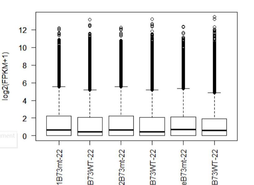
8.1以FPKM为参考值作图，以time作为区分条件

# 提取FPKM值

> fpkm = texpr(bg,meas="FPKM")

#方便作图将其log转换，+1是为了避免出现log2(0)的情况 > fpkm = log2(fpkm+1)

# 作图

>boxplot(fpkm,col=as.numeric(pheno_data$sex),las=2,ylab='log2(FPKM+1)')

图1

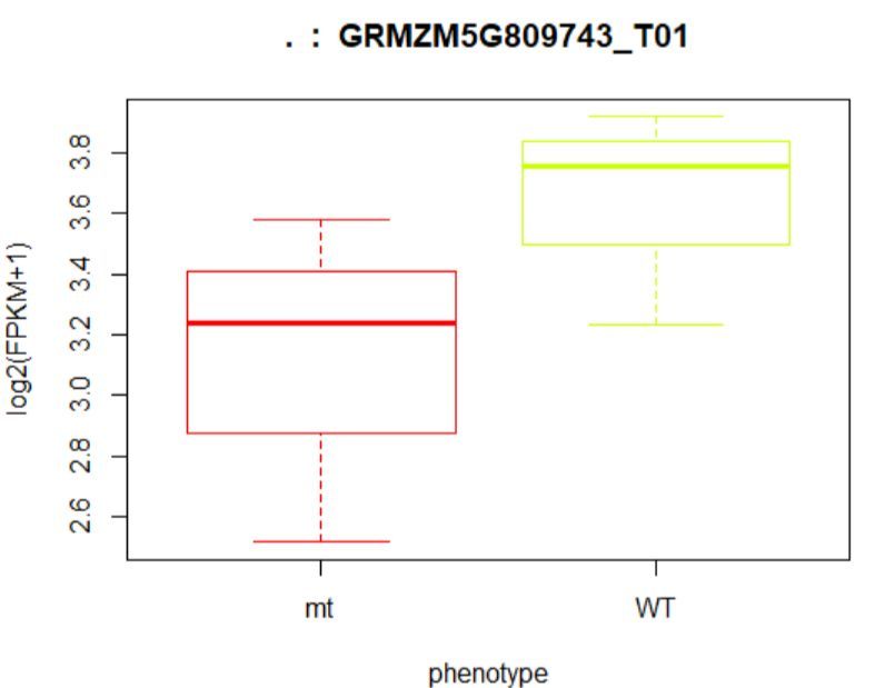
8.2就单个转录本的查看在样品中的分布

> ballgown::tranNames(bg)[12]

12 "NR_027232"

> ballgown::geneNames(bg)[12]

12 "LINC00685"

#绘制箱线图

> plot(fpkm[12,] ~ pheno_data$phenotype, border=c(1,2),

+ main=paste(ballgown::geneNames(bg)[12],' : ',

+ ballgown::tranNames(bg)[12]),pch=19, xlab="phenotype",

+ ylab='log2(FPKM+1)')

## (左图)

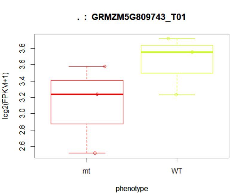
> points(fpkm[12,] ~ jitter(as.numeric(pheno_data$phenotype)),

+ col=as.numeric(pheno_data$phenotype))

## (右图)

8.3查看某一基因位置上所有的转录本

>plotTrans(ballgown::geneIDs(bg)[442], bg, main=c('Gene MSTRG.168 in sample sampleB73WT-22'), sample=c('sampleB73WT-22'))

有空格就出错 图2

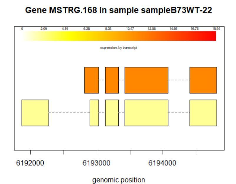
# plotTrans函数可以根据指定基因的id画出在特定区段的转录本

#可以通过sample函数指定看在某个样本中的表达情况，这里选用id=442, sample= sampleB73WT-22

> plotMeans('MSTRG.168',bg_filt,groupvar="phenotype",legend=FALSE)

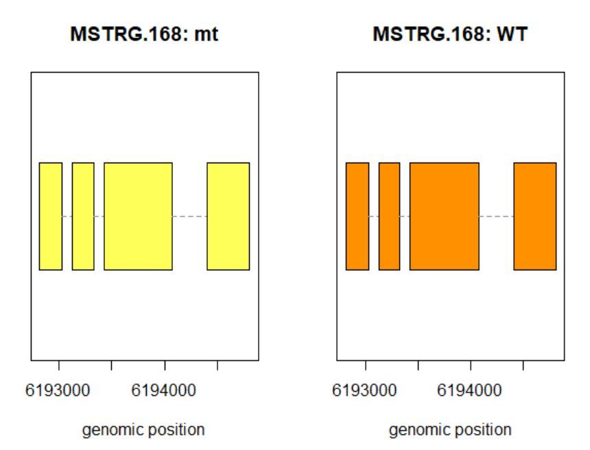
图3

最后编辑：2022-06-03

作者：萌小白

一个热爱网络的青年！

站内专栏 邮箱