学习章节

https://bioconductor.github.io/BiocWorkshops/r-and-bioconductor-for-everyone-an-introduction.html#introduction-to-bioconductor

文章目录

• 学习章节
• 1. Bioconductor的一些补充小用法
• 2. Working with Genomic Ranges
• 2.1 importing data 导入bed文件
• 2.2 Working with genomic ranges
• 2.3 Genomic annotations
• 2.4 Overlaps

1.Bioconductor的一些补充小用法

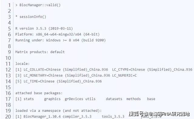
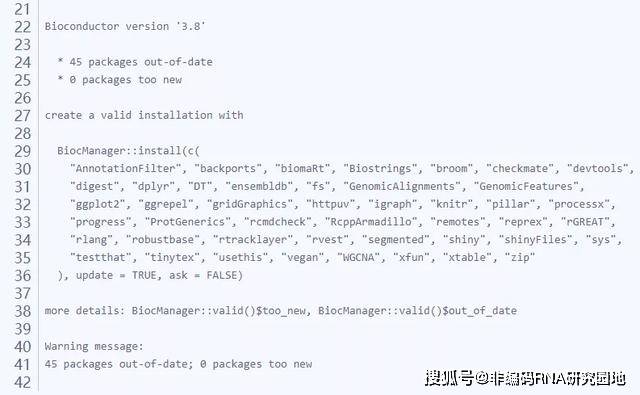
使用valid()查看包安装的版本情况

avaliable() 用于搜索相关的包

1 ## 例如这里输入TxDb.Hsapiens，它会自动匹配相关的包

2 BiocManager::available("TxDb.Hsapiens")

3 #> [1] "TxDb.Hsapiens.BioMart.igis"

4 #> [2] "TxDb.Hsapiens.UCSC.hg18.knownGene"

5 #> [3] "TxDb.Hsapiens.UCSC.hg19.knownGene"

6 #> [4] "TxDb.Hsapiens.UCSC.hg19.lincRNAsTranscripts"

7 #> [5] "TxDb.Hsapiens.UCSC.hg38.knownGene"

通过网站https://support.bioconductor.org/ 来查询解决和包相关的问题

2. Working with Genomic Ranges

• · Importing data
• · Working with genomic ranges
• · Genomic annotations
• · Overlaps

rtracklayer包提供函数import() 帮助用户读取基因组格式的文件(例如：BED,GTF,VCF,FASTA) 并封装成Bioconductor下的对象。GenomicRanges包提供了多种函数，来在基因组坐标系下操纵各种数据。

2.1 importing data 导入bed文件

1 library(rtracklayer)

2 ## 使用file.choose() 来选择文件

3 fname <- file.choose() # CpGislands.Hsapiens.hg38.UCSC.bed

4 fname

5 file.exists(fname)

6 ## 使用import()函数导入bed文件。导入后，将以GenomicRanges的对象描述这份CpG岛数据。

7 cpg <- import(fname)

8 cpg

注意 BED格式的文件，它们的坐标体系是0-based的，并且intervals是半开区间(start在范围内，end在范围后一个坐标里)

而Bioconductor得坐标是1-based，并且是闭区间(start和end坐标都包含在范围内)，因此使用import()函数导入数据得时候，它会自动将bed文件坐标转换为Bioconductor文件对象的坐标。

2.2 Working with genomic ranges

1 ## 使用函数 keepStandardChromosomes 保留标准染色体，标准染色体指的是chr1-22和x,y染色体

2 ## 很多时候我们获取的数据里 可能染色体不止chr1-22与x,y ；

3 ## 可能还包含其它染色体，例如：chr22_KI270738v1_random这样的染色体。

4 ## 通过keepStandardChromosomes 就可以去除这些其它的染色体，只保留标准染色体

5 cpg <- keepStandardChromosomes(cpg, pruning.mode = "coarse")

6 cpg

GenomicRanges对象包含两个部分

必需的：seqnames（染色体号），start（起始位点）,end(终止位点)，strand (正链或负链)

非必需的：另外的元素，例如本例中的name。

必需的元素内容，可以使用函数start(), end(), width()获取。非必需的元素，使用$符号获取内容。

1 head( start(cpg) )

2 #> [1] 155188537 2226774 36306230 47708823 53737730 144179072

3 head( cpg$name )

4

5 ## 使用subset()函数获取染色体1号和2号上的cpg岛

6 subset(cpg, seqnames %in% c("chr1", "chr2"))

2.3 Genomic annotations

1 ## 导入注释数据

2 library("TxDb.Hsapiens.UCSC.hg38.knownGene")

3 ## 查看注释数据中的所有转录本

4 tx <- transcripts(TxDb.Hsapiens.UCSC.hg38.knownGene)

5 tx

6 ## 为了演示方便，目前只保留标准染色体

7 tx <- keepStandardChromosomes(tx, pruning.mode="coarse")

8 tx

2.4 Overlaps

可以使用findOverlaps(),nearest(),precede()和follow()函数，来完成overlaps。

1 ## count the number of CpG islands that overlap each transcript

2 olaps <- countOverlaps(tx, cpg)

3 length(olaps) # 1 count per transcript

4 #> [1] 182435

5 table(olaps)

6 ## 将计算的overlaps加入GR对象

7 tx$cpgOverlaps <- countOverlaps(tx, cpg)

8 tx

9 ## subsetting the GRanges objects for transcripts satisfying particular conditions, in a coordinated fashion ## where the software does all the book-keeping to makes sure the correct ranges are selected.

10 subset(tx, cpgOverlaps > 10)

文章来源：Yujia_compbio

最后编辑：2022-12-16

作者：萌小白

一个热爱网络的青年！

站内专栏 邮箱